
Fracture response and local stress from microseismic data
Universal Seismic analyzes microseismic data recorded during hydraulic fracturing and geothermal stimulation. Fracture Imaging computes fracture geometry and conductivity from the event waveforms. Moment tensor and stress inversion resolve source mechanisms and the local stress field from the same data. We quantify how completion design, well spacing, and sequencing affect fracture response. Operators use the results to improve future completions.

Event locations vs. fracture response
In simulfrac and zipperfrac completions, event clouds from neighboring wells often overlap. Some events cannot be clearly assigned to a single well, so the fracture extent of each well remains poorly defined. Event locations provide no information on fracture conductivity.
Fracture Imaging produces high-resolution 3D fracture geometry and maps its more and less conductive parts. Our analytical workflow then separates the fracture surface area by well.


Completion and development decisions
Results are computed for each stage and grouped by design, well, formation, or zipper group. They are used to assess:
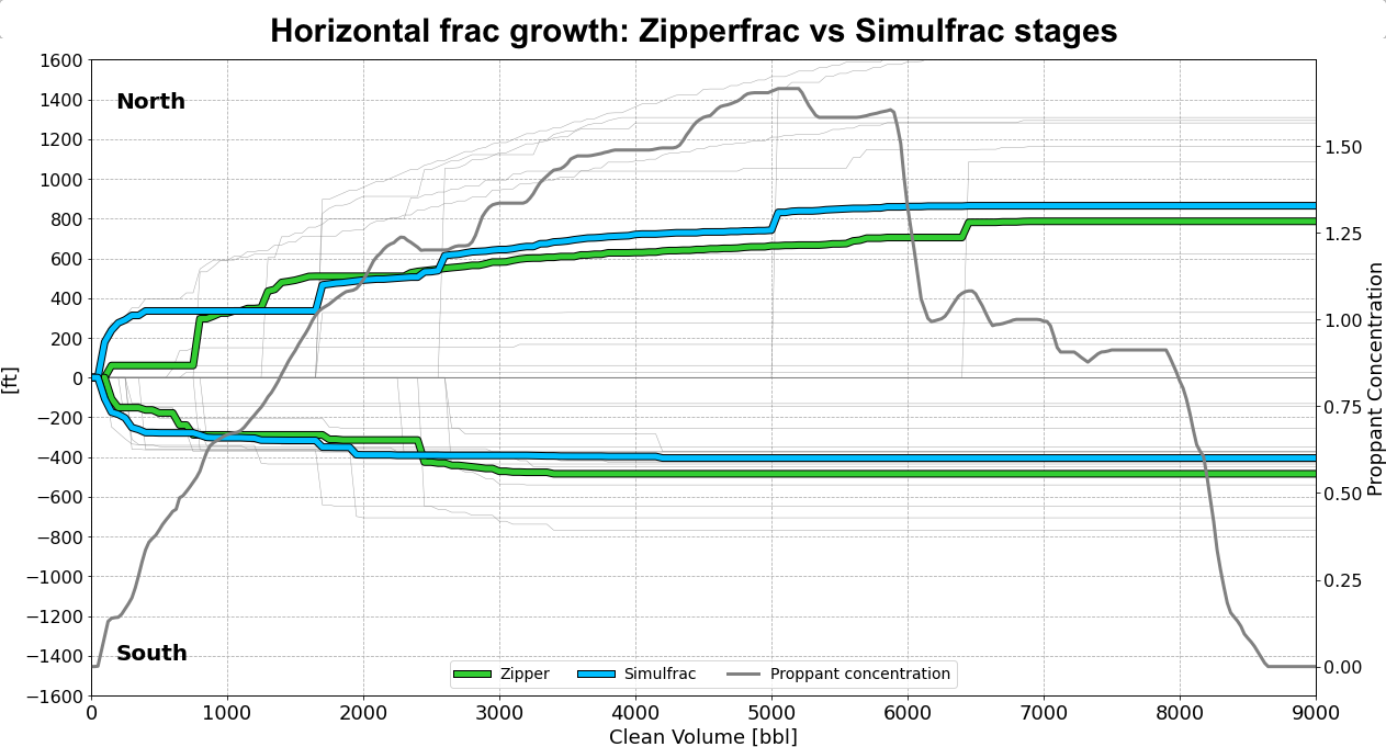
Completion design
Impact of each design on fracture surface area, conductivity, and fracturing efficiency
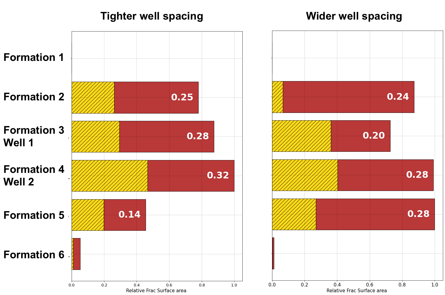
Well spacing
Impact of spacing on inter-well communication and lateral fracture extent
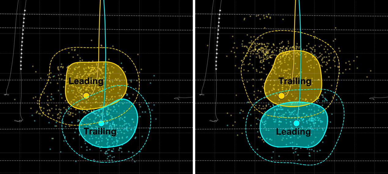
Sequencing
Impact of completion sequencing on total and conductive fracture growth
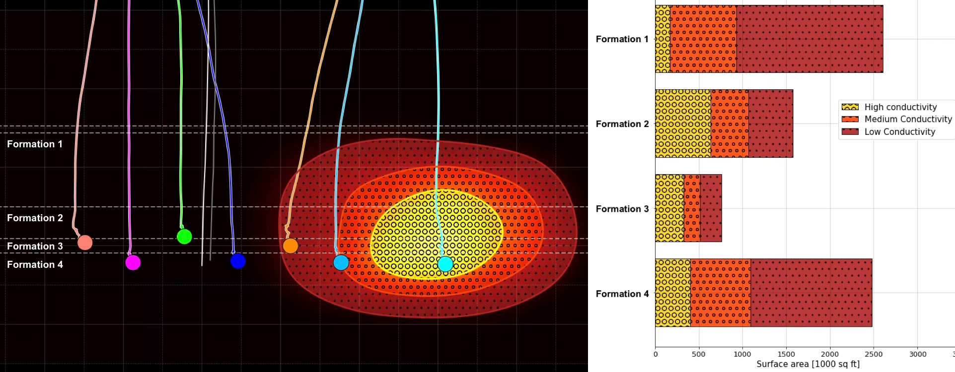
Landing interval
Impact of landing depth on height growth and fracture surface area by formation
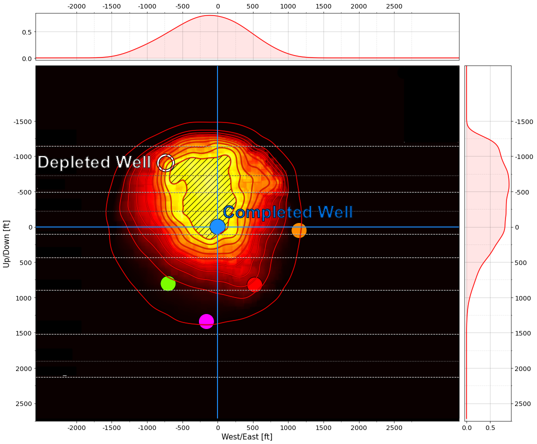
Depletion
Impact of depleted wells on fracture geometry and conductivity
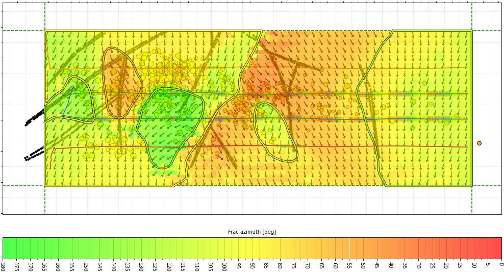
Local stress
Reactivation of pre-existing structures, stress interaction during simulfrac and zipperfrac operations, impact of perforation design on fracture initiation, and the local stress field around U-turn wells
Services
Each service can be contracted separately and applied to newly acquired and legacy datasets.
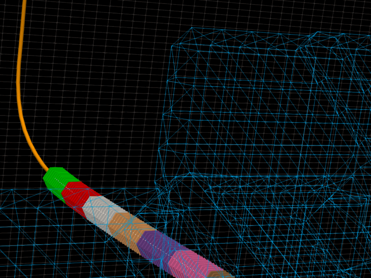
Fracture Imaging and analytics
Deliverables
Conductivity logs at cluster resolution, conductivity maps, fracture surface area by conductivity class, and stage-level metrics by design group →
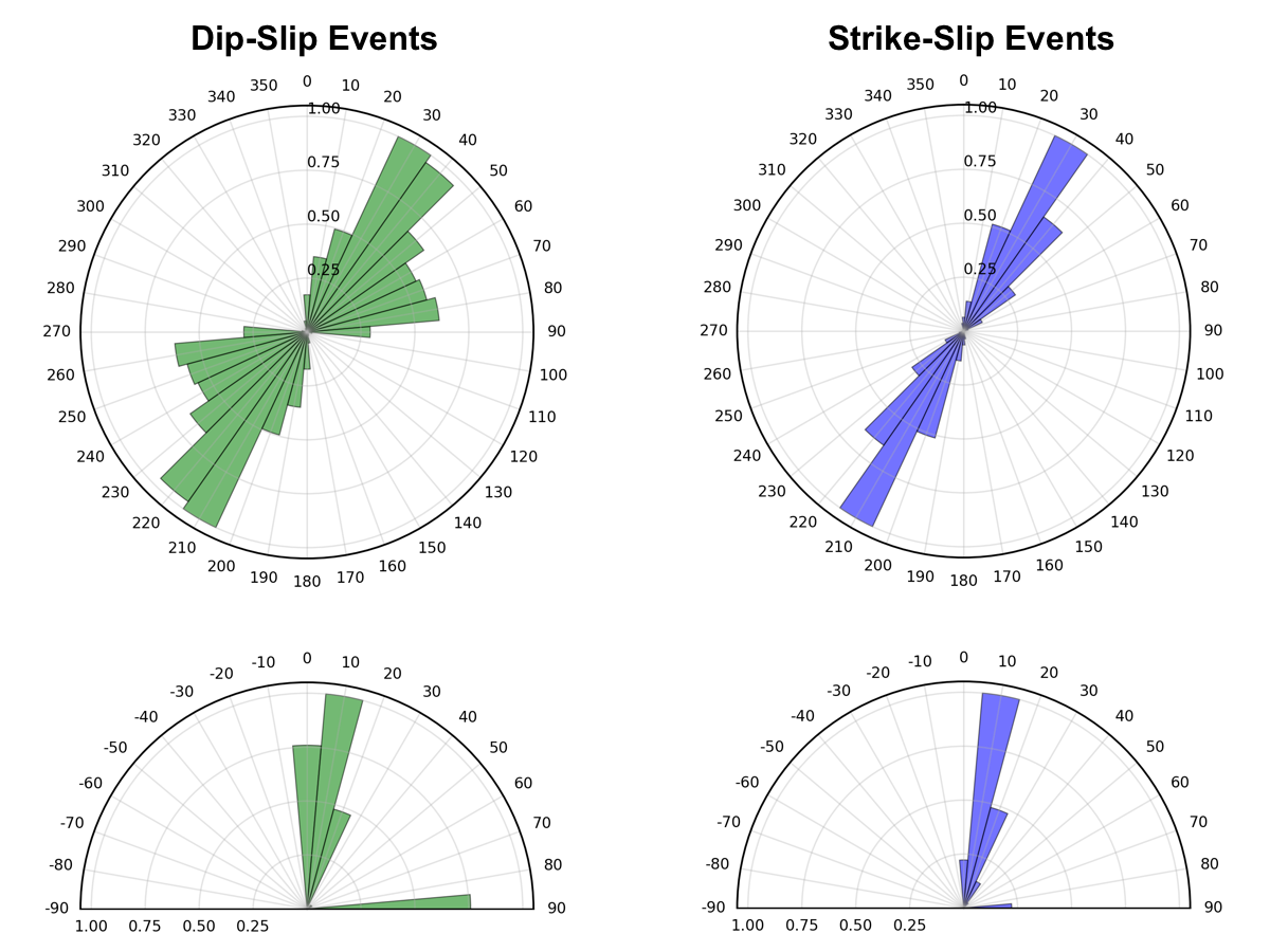
Moment tensor inversion
Deliverables
Moment tensor catalog, focal mechanisms, fault plane orientations, and stage rose diagrams →
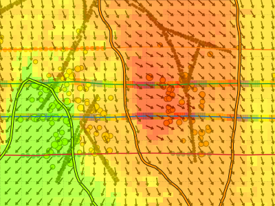
Stress inversion
Deliverables
3D effective stress field computed from the moment tensor catalog →


The required inputs are the velocity model, event locations, and event waveform records from baseline microseismic processing. Stress inversion requires moment tensor results. Projects that include several services receive joint analytics.
Validation and track record
Fracture Imaging was compared with fiber-optic data from two wells on HFTS2, a DOE-sponsored test site in the Delaware Basin (SPE-217815-MS, 2024). In the completed well, fiber strain data showed production flow at each cluster. An FI conductivity log was extracted from the 3D fracture image along the same well path and compared with the strain log. Fiber in a vertical offset well recorded fracture height growth.
- 99% clusters matched by an FI conductivity peak (115 of 116)
- ±6 ft agreement in cluster position
- 0.87 regression coefficient between normalized peak heights
- >2,000 ft upward growth recorded by fiber and imaged, not visible in event locations

The methods have been applied in multi-well projects for major operators in unconventional developments in North America. Several clients have commissioned repeat projects. The imaging method's first geothermal application was the Basel enhanced geothermal reservoir (Geophysics, 2015).
Validation details → · Paper (SPE-217815-MS) → · Publications →
How we work
All processing steps are documented and reproducible, so the client can verify every result. Fracture images include confidence volumes, and moment tensors include uncertainty estimates.
The client's team receives interim results throughout the project, and their questions guide the analysis. The people who developed the methods also work on the interpretation.